FLEXPART - Plotting cross sections

For preparations and running the simulation needed for this tutorial click here ...

The macro to plot a vertical cross section is 'plot_xs.mv'. We will see how this macro works.

First, we define the parameter and time step for the cross section then call flexpart_filter() to extract the data. The result is a fieldset with units of "kg m**-3", which we scale explicitly to "ng m**-3" units for plotting.

dIn="result_fwd/"
inFile=dIn  & "conc_s001.grib"

#Define level, parameter and step
lev=-1 #all levels
par="mdc" 
step=48

#Get fields for all levels for a given step
g=flexpart_filter(source: inFile,
                  param: par,
                  levType: "hl", 
                  step: step)

#Scale into ng/m3 units
g=g*1E12

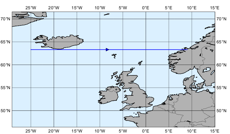
Next, we define the cross section view along this line:

xs_view = mxsectview(
	bottom_level	:	0,
	top_level	:	16000,
	line	:	[63.31,-25,63.31,9]
	)

Then, we define the contouring:

#The contour levels
cont_list=[1,10,50,100,150,200,250,500,750,1000,2000,5000,7000]

#Define contour shading
conc_shade = mcont(
	legend	:	"on",
	contour	:	"off",	
	contour_level_selection_type	:	"level_list",
	contour_level_list  : cont_list,
	contour_label	:	"off",
	contour_shade	:	"on",
	contour_shade_method	:	"area_fill",
	contour_shade_max_level_colour	:	"red",
	contour_shade_min_level_colour	:	"RGB(0.14,0.37,0.86)",
	contour_shade_colour_direction	:	"clockwise",	
    contour_method: "linear"
	)

and finally generate the plot:

plot(xs_view,g,conc_shade)

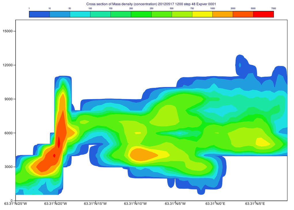
Having run the macro we will get a plot like this: