There are several ways on visualisating ODB data in Magics.
- use the ODB Magics objects. This allows Magics to read a odb file and extract some columns for geographical plots or graph.
- In python, it also possible to use odb_api packages to create a numpy array and pass the values in memeoty to Magics. magics is then able to perform symbol plotting on a geographical area, time series, etc ..
This page presents examples of visualisation, and offers skeletons of python programs.
To run the example at ECMWF:
- download python scripts and data
- module load Magics/new
- module load odb_api
Using an ODB file and create a geographical map
In this example, we have downloaded some ODB data from Mars.
The mars request looks like:
retrieve,
class = e2,
type = ofb,
stream = oper,
expver = 1607,
repres = bu,
reportype = 16005,
obstype = 1,
date = 20100101,
time = 0,
domain = g,
target = "data.odb",
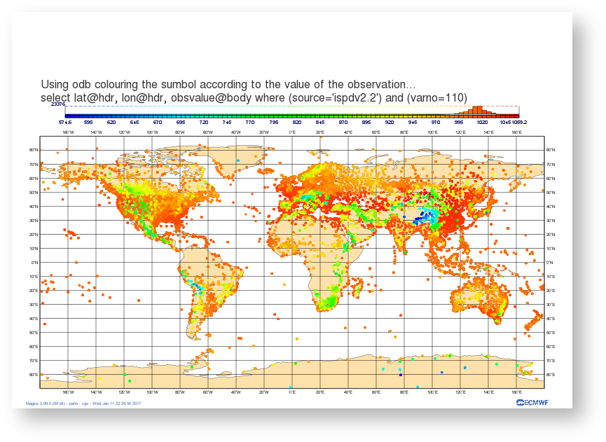
filter = "select lat@hdr, lon@hdr, obsvalue@body where (source='ispdv2.2') and (varno=110)",
duplicates = keep
We retrieve 3 columns lat@hdr, lon@hdr, obsvalue@body. In that case obsvalue@body will contain the value of the Surface pressure in Pascal.
We can dump the result :
lat@hdr         lon@hdr         obsvalue@body
84.559998       -44.100006      100180.000000
84.349998       -46.989990      100140.000000
83.610001       -89.299988      100380.000000
83.419998       -71.970001      100140.000000
83.300003       -69.040009      100090.000000
82.480003       -93.190002      100350.000000
82.449997       -170.309998     101510.000000
82.260002       -128.949997     99180.000000
81.449997       -144.850006     100180.000000
81.419998       -144.619995     100180.000000
81.400002       -145.550003     100250.000000
80.709999       -110.500000     100180.000000
80.320000       -179.860001     102969.992188
80.019997       -151.399994     100440.000000
In this example, we will ask Magics to load this ODB file, and plot the position of each observation using the simple marker. WE have to inform Magics about the name of the columns to use to find the latitude, and longitude information.

Download :
Now, we are going to colour the symbol according to the value of the observation. The advanced mode for symbol plotting offers an easy way to specify range and colours, we add a legend for readability.

Download :
Loading the data into a numpy array and passing them to Magics
Note the facilities offered by numpy to perform some computations and the histogram legend facilities of Magics.
Download :
Creating a time series from an ODB data.
In this example, we will first setup a cartesian projection for the time series: the x axis will show the date from January 2005 to December 2010, and the y axis will represent the number of observation for each day, i.e. a range from 0 to 1000.
This plot needs the creation of 3 Magics objects a mmap to describe the projection and 2 axis to specify labels, ticks and other attributes.
The plot command will create a png showing the projection represented by the 2 axis.

Note the use of axis_type = 'date', axis_date_type = "automatic" in the setting of the horizontal axis. This is a nice feature of Magics that will adjust the labels to show hours, days, months or years according to the length of the time series.
Now we will add the data. The file count.odb contains the following information.
date@hdr	series
20041231	7124.000000
20050101	112191.000000
20050102	117146.000000
20050103	118529.000000
20050104	115592.000000
20050105	115085.000000
20050106	112501.000000
20050107	116017.000000
20050108	118702.000000
20050109	117507.000000
20050110	119497.000000
We will first try to create a basic curve considering the date as a integer.

Note that we have now set subpage_x_axis_type to regular and subpage_x_automatic = on. This will not interpret the date as a date but as a integer, and will use the min and max of the data to setup the limits of the projection. It is not the plot we really want, but it gives a quick overview.
Download :
Let's nterpret the date as date, and the time series should be fine.

Download :
In the example we are using numpy array to manipulate the ODB, this gives all the computations facilities. Once done, the result can just be passed to Magics using through a numpy array.