Page History
| Section | ||||||||||||
|---|---|---|---|---|---|---|---|---|---|---|---|---|
|
...
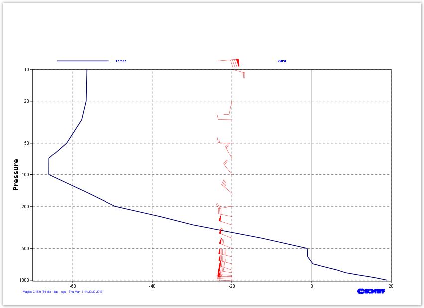
- a horizontal regular axis for a temperature range going from -60oC to 20oC.
- a vertical logarithmic axis going from 1020 hPa to 10 hPa
Have a look at the Subpage Documentation and at the Axis Plotting Documentation, and try to get the 0oC grid line highlighted.
...
We want to plot these winds as red falgs flags on the vertical of -20.
The mgraph object can then be used to to preform the visualisation. All the parameters can be found in the Graph Plotting Page.
Do not forget the to add a legend with a some meaningful text!
| Section | |||||||||||||||||||||||||||||||||||||
|---|---|---|---|---|---|---|---|---|---|---|---|---|---|---|---|---|---|---|---|---|---|---|---|---|---|---|---|---|---|---|---|---|---|---|---|---|---|
|
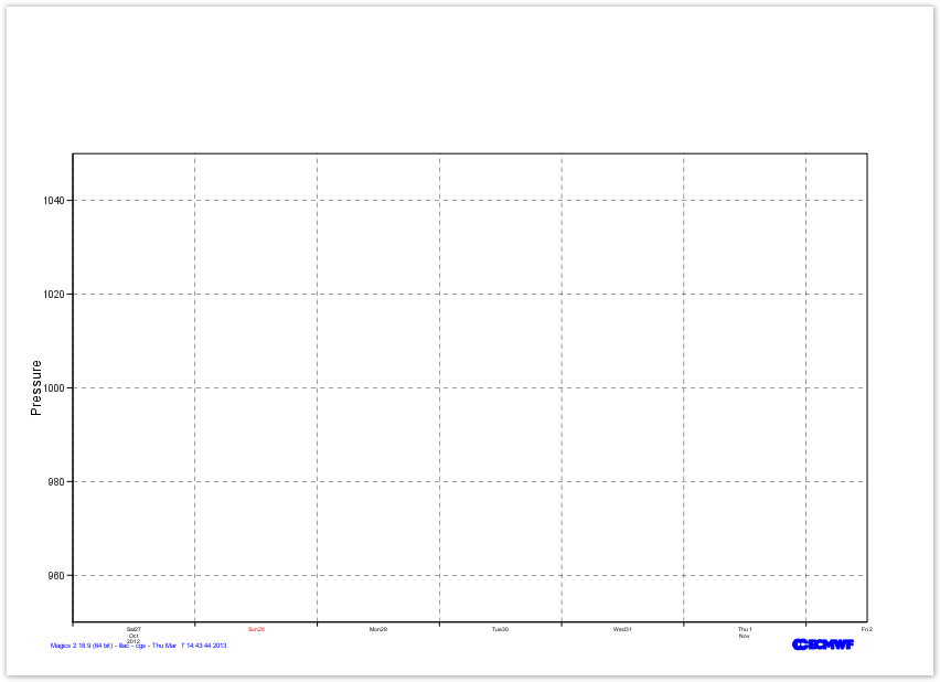
Time Series: Setting the Cartesian Projection for the Mean Sea Level Pressure time series
In this exercise, we will learn how to setup a date Coordinate, and browse the parameters available to style the style a date axis.
We want
- a horizontal date axis going from the 2012-10-27at 00:00:00 to 2012-11-02 12:00:00
- a vertical regular axis going from 950 hPa to 1005 hPa
Have a look at the Subpage Documentation and at the Axis Plotting Documentation,
|
Time Series: Setting the Cartesian Projection for the Mean Sea Level Pressure time series
In this exercise, we will learn how to setup a date Coordinate, and browse the parameters available to style the style a date axis.
We want
- a horizontal date axis going from the 2012-10-27at 00:00:00 to 2012-11-02 12:00:00
- a vertical regular axis going from 950 hPa to 1050 hPa
Have a look at the Subpage Documentation and at the Axis Plotting Documentation,
| Section | |||||||||||||||||||||||||||||||||||||
|---|---|---|---|---|---|---|---|---|---|---|---|---|---|---|---|---|---|---|---|---|---|---|---|---|---|---|---|---|---|---|---|---|---|---|---|---|---|
|
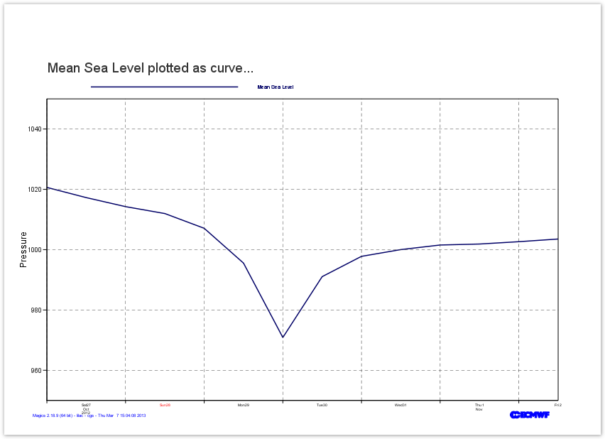
Time Series: Using a CSV file as input of a curve
The values for our time series are in CSV (Comma-Separeted-Value) ascii file called msl.csv.
| Code Block | ||
|---|---|---|
| ||
1,2012-10-27 00:00:00,1020.64125,0
2,2012-10-27 12:00:00,1017.261875,0.1220703125
3,2012-10-28 00:00:00,1014.27125,-9.58071727163e-21
4,2012-10-28 12:00:00,1011.97375,-2.80979885101e-20 |
The valid date is defined in the second column, the value of msl in the third.
This information need to be given to Magics . This can be done with the mtable data action,. See the full documentation.
The mgraph action will then be used to define the curve attributes. All the parameters can be found in the Graph Plotting Page.
You can always add a title using the mtext object.
| Section | ||||||||||||||||||||||||||||||||||||
|---|---|---|---|---|---|---|---|---|---|---|---|---|---|---|---|---|---|---|---|---|---|---|---|---|---|---|---|---|---|---|---|---|---|---|---|---|
| ||||||||||||||||||||||||||||||||||||
| Section | ||||||||||||||||||||||||||||||||||||
|
Time Series: Using a CSV file as input of a curve
The values for our time series are in CSV (Comma-Separeted-Value) ascii file called msl.csv.
| Code Block | ||
|---|---|---|
| ||
1,2012-10-27 00:00:00,1020.64125,0
2,2012-10-27 12:00:00,1017.261875,0.1220703125
3,2012-10-28 00:00:00,1014.27125,-9.58071727163e-21
4,2012-10-28 12:00:00,1011.97375,-2.80979885101e-20 |
The valid date is defined in the second column, the value of msl in the third.
This information need to be given to Magics . This can be done with the mtable data action.
The mgraph action will the be used to define the curev attributes. All the parameters can be found in the Graph Plotting Page.
You can always add a title using the mtext object.
...
| width | 50% |
|---|
...
| title | Parameters to check |
|---|
|
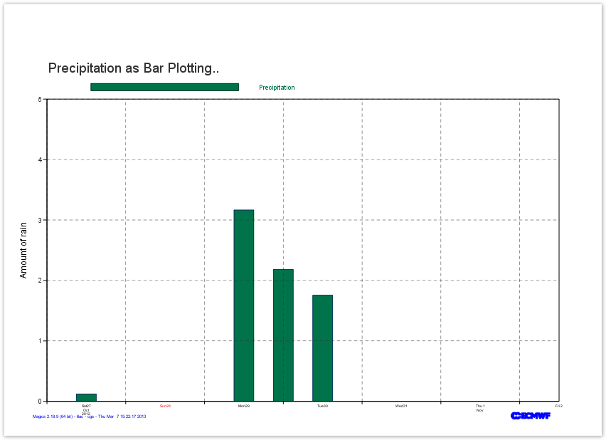
Time Series : Using Automatic Axis and bar plotting
Magics can automatically set-up the coordinates system according to the plotted data.
In this exercise, we will use this functionality to draw the time series of the precipitation.
- The horizontal date coordinate system is set automatically.
- The vertical coordinate system is regular going from 0 to 5
The data will be pass to Magics using arrays:
dates = ["2012-10-27 00:00:00","2012-10-27 12:00:00","2012-10-28 00:00:00", "2012-10-28 12:00:00","2012-10-29 00:00:00","2012-10-29 12:00:00", "2012-10-30 00:00:00","2012-10-30 12:00:00", "2012-10-31 00:00:00","2012-10-31 12:00:00", "2012-11-01 00:00:00","2012-11-01 12:00:00", "2012-11-02 00:00:00","
| Useful table parameters |
|---|
table_filename |
| table_variable_identifier_type |
| table_x_type |
| table_x_variable |
| table_y_variable |
| table_header_row |
| Useful graph parameters |
|---|
| graph_line_colour |
| legend |
| legend_user_text |
...
| theme | Confluence |
|---|---|
| language | python |
| title | Python - Input data and Flags plotting |
| collapse | true |
...
2012-11-02 12:00:00"]
precip = [0.,0.1220703125,0.,0., 0., 3.16429138184, 2.18200683594,1.75476074219,0,0,0,0,0,0.]We want to display the information using bar plotting.
We will perhaps need to check quickly
- The Subpage Documentation
- The Axis Documentation
- The Input Data Documentation
- The Graph Plotting Documentation
| Section | |||||||||||||||||||||||||||||||||||||||
|---|---|---|---|---|---|---|---|---|---|---|---|---|---|---|---|---|---|---|---|---|---|---|---|---|---|---|---|---|---|---|---|---|---|---|---|---|---|---|---|
|
Time Series : Using Automatic Axis and bar plotting
Magics can automatically set-up the coordinates system according to the plotted data.
In this exercise, we will use this functionality to draw the time series of the precipitation.
- The horizontal date coordinate system is set automatically.
- The vertical coordinate system is regular going from 0 to 5
The data will be pass to Magics using arrays:
...
|
...
|
...
|
...
|
...
|
...
|
...
|
...
|
...
|
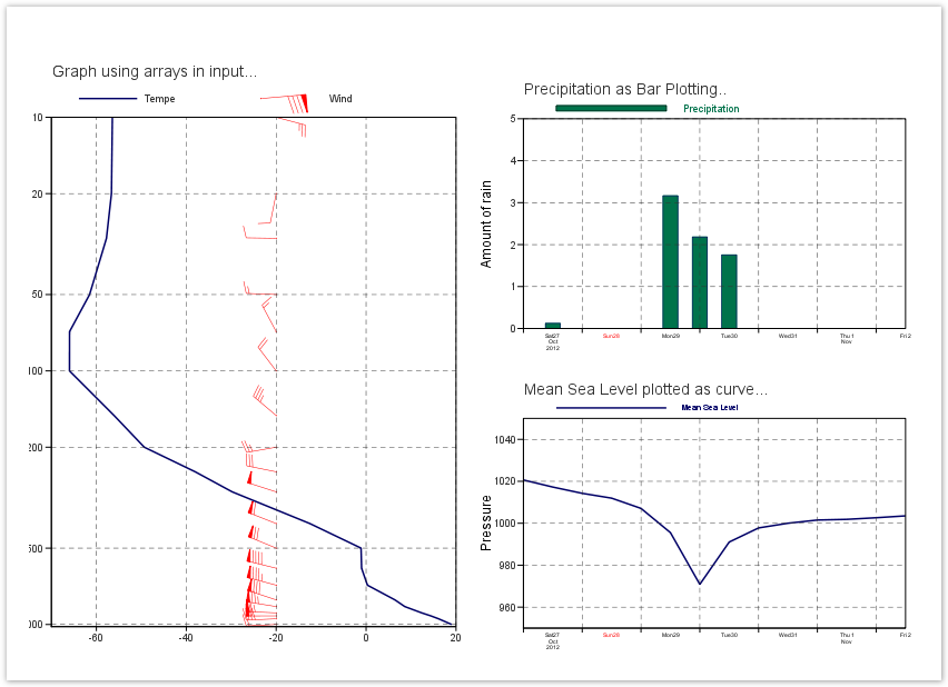
Finally, A bit of layout ...
On our image, we want to create 3 pages.. We will use the pseudo action page to do that..
| Gliffy Diagram | ||
|---|---|---|
|
The position of the page is set with the 4 following parameters
- page_x_position / page_y_position : to position in cm the bottom left corner of the page in its parent
- page_x_length / page_y_length : the dimension in cm.
The drawing area ( where the plotting is rendered) is called subpage and can position into the page using the 4 following parameters
- subpage_x_position / subpage_y_position : to position in cm the bottom left corner of the drawing area (subpage) in its parent page.
- subpage_x_length / subpage_y_length : the dimension in cm.
| Section | |||||||||||||||||||||||||||||||||
|---|---|---|---|---|---|---|---|---|---|---|---|---|---|---|---|---|---|---|---|---|---|---|---|---|---|---|---|---|---|---|---|---|---|
|
"2012-10-30 00:00:00","2012-10-30 12:00:00", "2012-10-31 00:00:00","2012-10-31 12:00:00", "2012-11-01 00:00:00","2012-11-01 12:00:00", "2012-11-02 00:00:00","2012-11-02 12:00:00"]precip = [0.,0.1220703125,0.,0., 0., 3.16429138184, 2.18200683594,1.75476074219,0,0,0,0,0,0.]We want to display the information using bar plotting.
We will perhaps need to check quickly
- The Subpage Documentation
- The Axis Documentation
- The Input Data Documentation
- The Graph Plotting Documentation
| Section | ||||||||||||||||||||||||||||||||||||||||
|---|---|---|---|---|---|---|---|---|---|---|---|---|---|---|---|---|---|---|---|---|---|---|---|---|---|---|---|---|---|---|---|---|---|---|---|---|---|---|---|---|
|