For preparations and running the simulation needed for this tutorial click here ...
| Note |
|---|
To start these this tutorial please enter folder 'forward'. |
...
First, we define the parameter and time step for the cross section then call flexpart_filter() to extract the data. The result is a fieldset with units of "kg m**-3" that , which we need to scale explicitly convert to "ng m**-3" units for plotting since the automatic units scaling only works for map based plots.
| Code Block | ||
|---|---|---|
| ||
dIn="result_fwd/" inFile=dIn & "conc_s001.grib" #Define level, parameter and step lev=-1 #all levels par="mdc" step=48 #Get fields for all levels for a given step g=flexpart_filter(source: inFile, param: par, levType: "hl", step: step) #Scale into ng/m3 units g=g*1E12 |
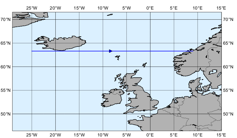
Next, we define the cross section view along this line:
...
| language | py |
|---|
...
,
...
Then, we define the contouring:
| Code Block | ||||||
|---|---|---|---|---|---|---|
| ||||||
#The contour levels
cont_list=[1,10,50,100,150,200,250,500,750,1000,2000,5000,7000]

#Define contour shading
conc_shade = mcont(
	legend	:	"on",
	contour	:	"off",
	contour_level_selection_type	:	"level_list",
	contour_level_list  : cont_list,
	contour_label	:	"off",
	contour_shade	:	"on",
	contour_shade_method	:	"area_fill",
	contour_shade_max_level_colour	:	"red",
	contour_shade_min_level_colour	:	"RGB(0.14,0.37,0.86)",
	contour_shade_colour_direction	:	"clockwise",
    contour_method: "linear"
) |
Then, we define the cross section view along this line:
| Code Block | ||
|---|---|---|
| ||
xs_view = mxsectview( bottom_level : 0, top_level : 16000, line : [63.31,-25,63.31,9] ) |
and finally generate the plot:
...
