...
| Gliffy Diagram | ||||
|---|---|---|---|---|
|
Exercise 1.
...
The ECMWF analysis
Handout
See map of observations of wind-gust during the storm and the timeseries of maximum gusts.
...
| Info | ||
|---|---|---|
| ||
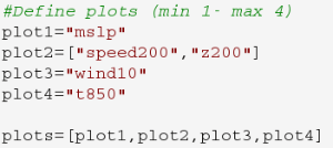
For the an_2x2.mv icon the number of maps appearing in the plot layout can be 1, 2, 3 or 4. This is true of all the icons labelled '2x2'.
Right-click on the icon and select 'Edit'. Change the plot layout like this:
Note how some plots can be single parameters whilst others can be overlays of two (or more) fields. Wind parameters can be shown either as arrows or as feather by adding '_f' to the variable name. Two map types are available covering a different area.
With mapType=0, the map will cover a smaller geographical area centred on the UK. With mapType=1, the map will cover most of the North Atlantic |

Exercise 2:
...
The operational HRES forecast
Recap
The ECMWF operational deterministic forecast is called HRES. The model runs at a spectral resolution of T1279, equivalent to 16km grid spacing.
...
| Note | |||||
|---|---|---|---|---|---|
| |||||
Task 1: Forecast errorRoot-mean square error curves are often used to determine forecast error compared to the analysis. In this task, all 4 forecast dates will be used. Using the oper_rmse.mv icon, right-click, select 'Edit' and plot the RMSE curves for MSLP (mean-sea-level pressure) & wgust10 (10m wind gust). Repeat for both geographical regions: mapType=0 and mapType=1. Q. What do the RMSE curves show? Task 2: Compare forecast to analysisUse the oper_to_an_runs.mv icon (right-click -> Edit) and plot the MSLP and wind fields. This shows a comparison of each of the forecasts to the analysis. Use the oper_to_an_diff.mv icon and plot the difference map between a forecast date and the analysis.
Task 3: Team workingAs a team, discuss the plots & parameters to address the questions above given what you see in the error growth curves and maps from task 2. Look at the difference between forecast and analysis to understand the error in the forecast, particularly the starting formation and final error. Team members can look at particular dates and choose particular variables for team discussion. Remember to save (or print) plots of interest for later group discussion. |
Exercise 3 :
...
The operational ensemble forecasts
...
Recap
- Sources of forecast uncertainty: initial analysis and model error.
- Initial analysis uncertainty: sampled by use of Singular Vectors (SV) and Ensemble Data Assimilation (EDA).
- Model uncertainty: sampled by use of stochastic processes. In IFS this means Stochastically Perturbed Physical Tendencies (SPPT) and the spectral backscatter scheme (SKEB)
- Singular Vectors: a way of representing the fastest growing modes.
- Ensemble mean : the average of all the ensemble members. Where the spread is high, small scale features can be smoothed out in the ensemble mean.
- Ensemble spread : the standard deviation of the ensemble members and represents how different the members are from the ensemble mean.
...