...
Saving images and printing
...
To save images during these exercises for discussion later, you can use:
| Panel | ||
|---|---|---|
| ||
"Export" button in Metview's display window under the 'File' menu. This will also allow animations to be saved into postscript. |
or
| Code Block | ||||
|---|---|---|---|---|
| ||||
ksnapshot |
| Info | ||
|---|---|---|
| ||
. If hardcopy prints are desired please use the printer at the rear of the classroom and only print if necessary. |
...
| Panel | ||||
|---|---|---|---|---|
| ||||
The case study will look at one of several severe wind-storms that hit Europe in late 2013 (see handout of ECMWF article by Hewson et al, ECMWF Newsletter 139).
|
Outline of exercisesof exercises
The following schematic shows the flow of the 4 exercises.
We start by looking at the analyses to understand the development and behaviour of the storm. Then we look at the operational ECMWF forecast before then looking at the operational ensemble performance. Finally, the last exercise explores the role and impact of changing the degree of uncertainty represented in the forecasts.
| Gliffy Diagram | ||||
|---|---|---|---|---|
|
...
How to plot in various layouts
...
...
Icon 'an_1x1.mv' produces a single plot on the page.
Icon 'an_2x2.mv' can produce up to 4 plots per page.
| Info | |||
|---|---|---|---|
| Change plot fields
| ||
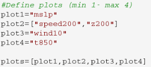
For the To alter the plotted field, right-click and choose It is possible to overlay multiple fields by putting them in square brackets like this:
You will find a list of available parameters in the macro. After editing the macro text, you can optionally save using the 'File' menu and 'Save'. Display the plot by clicking: Animate the plots in the display window by clicking |

| Info | |||
|---|---|---|---|
| Change
| ||
For the an_2x2.mv icon the number of maps appearing in the plot layout can be 1, 2, 3 or 4. This is true of all the icons labelled '2x2'.
Right-click on the icon and select 'Edit'. Change the plot layout like this:
Note how some plots can be single parameters whilst others can be overlays of two (or more) fields. Wind parameters can be shown either as arrows or as feather by adding '_f' to the variable name. Two map types are available covering a different area.
With mapType=0, the map will cover a smaller geographical area centred on the UK. With mapType=1, the map will cover most of the North Atlantic |

Exercise 2: Visualise operational HRES forecast
Recap
...
The ECMWF operational deterministic forecast is called HRES. The model runs at a spectral resolution of T1279, equivalent to 16km grid spacing.
Only a single forecast is run at this resolution as the computational resources required are demanding. The ensemble forecasts are run at a lower resolution.
Before looking at the ensemble forecasts, first understand the performance of the operational HRES forecast.
Available forecast dates
...
Data is provided for multiple forecasts starting from different dates, known as different lead times.
Available lead times for the St Judes storm are forecasts starting from these October 2013 dates: 24th, 25th, 26th and 27th.
Some tasks will use all the lead times, others require only one.
Available plot types
| Panel |
|---|
For this exercise, you will use the metview icons in the row labelled 'Oper forecast' as shown above. oper_rmse.mv : this plots the root-mean-square-error growth curves for the operational HRES forecast for the different lead times.
oper_to_an_runs.mv : this plots the same parameter from the different forecasts for the same verifying time. Use this to understand how the forecasts differed, particularly for the later forecasts closer to the event. oper_to_an_diff.mv : this plots a single parameter as a difference between the operational HRES forecast and the ECMWF analysis. Use this to understand the forecast errors from the different lead times.
Parameters & map appearance. These macros have the same choice of parameters to plot and same choice of |
...