...
| Panel | ||||||
|---|---|---|---|---|---|---|
| ||||||
The case study will look at one of several severe wind-storms that hit Europe in late 2013 (see handout of ECMWF article by Hewson et al, ECMWF Newsletter 139).
|
Recap
Key points
- Sources of forecast uncertainty: initial analysis and model error.
- Initial analysis uncertainty: sampled by use of Singular Vectors (SV) and Ensemble Data Assimilation (EDA).
- Model uncertainty: sampled by use of stochastic processes. In IFS this means Stochastically Perturbed Physical Tendencies (SPPT) and the spectral backscatter scheme (SKEB)
ECMWF operational forecasts consist of:
- HRES : T1279 (16km grid) highest resolution 10 day forecast
- ENS : Ensemble (50 members), T639 for days 1-10, T319 days 11-15.
| Panel | ||||||
|---|---|---|---|---|---|---|
| ||||||
We suggest these exercises are best done by small groups working in teams. Suggestions are made in the exercises for how each team can work on different data. |
Exercise 1. Evaluating the ECMWF analyses and forecasts
Objective: Understanding (a) formation of the storm (b) the error in the forecast by comparing the ECMWF forecast with analysis & observations
Starting up metview
| Code Block | ||
|---|---|---|
| ||
metview |
| Info |
|---|
Please enter the folder 'OpenIFS workshop 2015' to begin working. |
Task 1: Visualise observations and ECMWF analyses
| Panel | ||||||
|---|---|---|---|---|---|---|
| ||||||
For this task, use the metview icons in the row labelled 'Analysis'
|

| Panel | ||||||
|---|---|---|---|---|---|---|
| ||||||
1. Right-click on the icon labelled ' |
| Panel | ||||||
|---|---|---|---|---|---|---|
| ||||||
For this task, use the metview icons in the row labelled 'Analysis'
|
| Panel | ||||||
|---|---|---|---|---|---|---|
| ||||||
1. Right-click on the icon labelled ' |
| ||||||||||
Icon ' Icon | ||||||||||
| Panel | ||||||||||
|---|---|---|---|---|---|---|---|---|---|---|
| ||||||||||
Icon ' Icon
|


| Note | ||||
|---|---|---|---|---|
| ||||
|
| Note | ||||
|---|---|---|---|---|
| ||||
If you prefer to see multiple plots per page rather than overlay them, please use the |
Task 2: Visualise operational HIRES forecast
...
| Panel | ||||||
|---|---|---|---|---|---|---|
| ||||||
The ECMWF operational forecast is called HIRES. The model runs at a spectral resolution of T1279, equivalent to 16km grid spacing. Only a single forecast is run at this resolution as the computational resources required are demanding. The ensemble forecasts are run at a lower resolution. Before looking at the ensemble forecasts, first understand the performance of the HIRES forecast. | ||||||
| Panel | ||||||
| ||||||
. Only a single forecast is run at this resolution as the computational resources required are demanding. The ensemble forecasts are run at a lower resolution. Before looking at the ensemble forecasts, first understand the performance of the HIRES forecast. |
| Panel | ||||||
|---|---|---|---|---|---|---|
| ||||||
Data is provided for multiple forecasts starting from different dates, known as different lead times. Available lead times for October 2013 are: 24th, 25th, 26th and 27th. |
| Panel | ||||||
|---|---|---|---|---|---|---|
| ||||||
For this task, use the metview icons in the row labelled 'Oper forecast'
oper_to_an_runs.mv plots the same parameter from the different forecasts for the same verifying time. Use this to understand how the forecasts differed, particularly for the later forecasts closer to the event. oper_to_an_diff.mv plots a single parameter as a difference between the operational HIRES forecast and the ECMWF analysis. Use this to understand the forecast errors from the different lead times. |

Use the metview macros to plot different days and compare to analysis and plot forecast differences.
| Note | ||||
|---|---|---|---|---|
| ||||
|
| Notepanel | |||||||
|---|---|---|---|---|---|---|---|
| |||||||
For this task, use the metview icons in the row labelled 'Oper forecast'
|

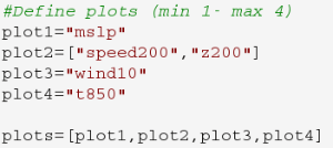
Suggested fields to plot: MSL, Z200, 10m wind and visualize the storm track.
Use the metview macros to plot different days and compare to analysis and plot forecast differences.
...
| ||
Each team should look at the forecast from all 4 starting dates. As a team, discuss what plots & parameters to use to address the questions above. A starting point is to look at the difference between forecast and analysis to understand the error in the forecast, particularly the starting formation and final error. Team members can look at particular dates and choose particular variables for team discussion. |
Task 2 : Visualize the ensemble forecasts and ensemble spread
Recap
Key points
- Sources of forecast uncertainty: initial analysis and model error.
- Initial analysis uncertainty: sampled by use of Singular Vectors (SV) and Ensemble Data Assimilation (EDA).
- Model uncertainty: sampled by use of stochastic processes. In IFS this means Stochastically Perturbed Physical Tendencies (SPPT) and the spectral backscatter scheme (SKEB)
Again using the ECMWF operational forecast, look now at the 50 ensemble forecasts. These are at a lower resolution (T639) than the HIRES (T1279).
...
Exercise 2. CDF/RMSE at different locations
Recap
TO DO: RMSE & CDF (concepts need explanation)
...