Page History
...
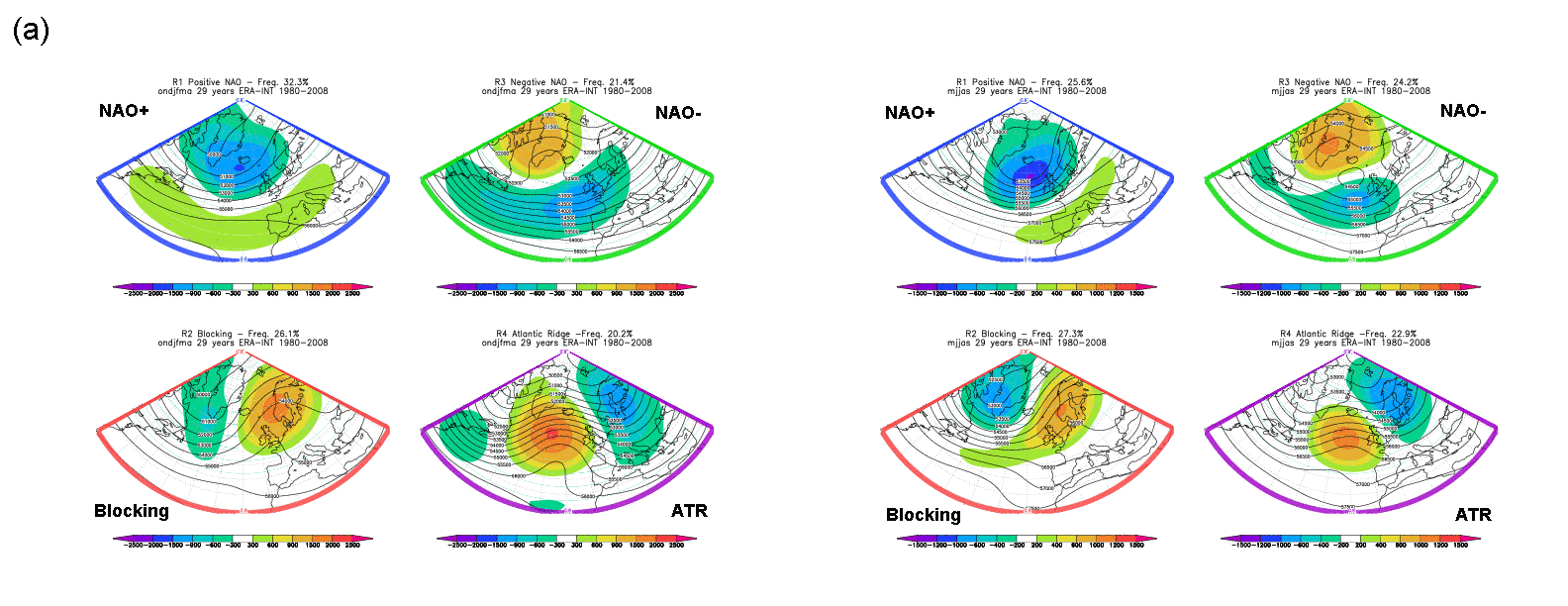
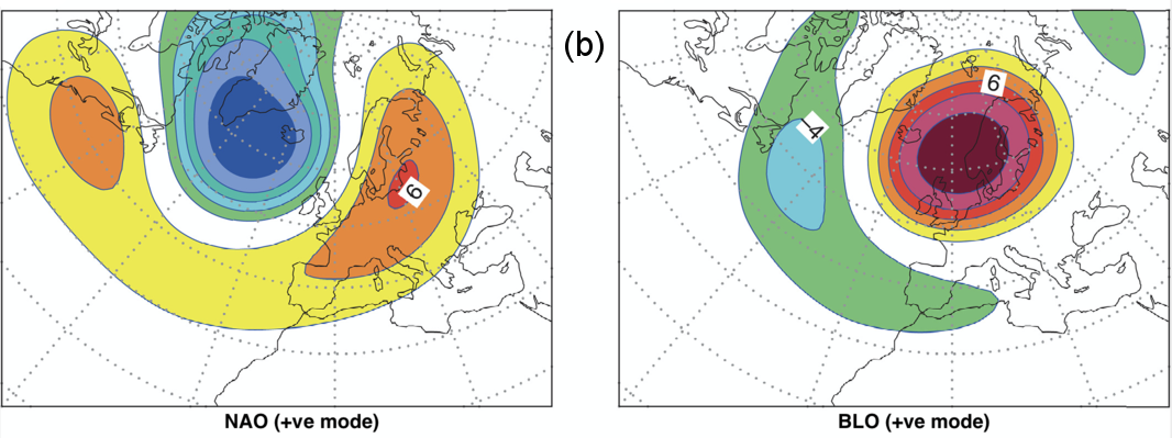
Regime assignment of forecast data is in each case computed in Empirical Orthogonal Function (EOF) space using "calibrated" anomalies of 500mb height/geopotential. These anomalies are computed with respect to the re-forecast 20-year climate (ER-M-climate), and then those anomalies are compared with reference points for the regime definitions (that are themselves based on re-analysis data) in order to achieve regime assignment. Fig8.1.15.1A and Fig8.1.15.1B Fig74.A and Fig74.B show what these regime reference points look like in 500mb anomaly space for the two schemes. These are for illustrative purposes only – the user should not expect a model forecast assigned to a particular regime to look exactly like these; ordinarily there will just be some vague resemblance.
For the 4-regime scheme, whilst two sets of anomalies are shown, in reality the reference points against which forecast anomalies are compared actually vary smoothly through the year. This is done by giving different weights to these patterns depending upon the month. So for forecasts for the main months of winter and of summer the reference points will be almost identical to that shown in, respectively, the left and right sets in Fig8.1.15.1AFig74.A, whilst for intermediate month forecasts they will be a weighted combination.
...
Fig8.1.15.1BFig74.B: Diagrams depict the Euro-Atlantic sector around which the regime definitions used in ECMWF products are based.
...

